Matatus; Route Planning Using Neo4J

I have, for a year now, been trying to make an Opensource matatu transit application on Android for Nairobi. I must say, it has not been easy. I made some bad decisions. Some that have lead to me barking on the provabial wrong tree. I will, in this blog post, expound on one of the mistakes I made, my initial reasoning behind making this ‘silly’ decision and why I was wrong.

The Android app was initially inteded to be fully functional offline. I wanted to make it this way because my assumption was that the path selection problem for this particular case was going to be trivial (or trivial enough to run comfortably on any device). The users, definated, would have also appreciated an offile application. The consequences of making the application offline were:

1. I’d have to cache the entire GTFS dataset. That really wasn’t a problem. The entire dataset was roughly 1.5M on the wire and 3M when dumped in an SQLite database on the device. Copying the entire dataset into an object in memory also didn’t take long. I didn’t bother breaking up the GTFS into chunks because this was the first prototype and I just wanted to make things work first.

2. The entire path selection algorithm had to be handled on the device. The agorithm was able to calculate relatively complex paths. It however took quite a bit of time calculating the more complex paths. More of this in the next paragraphs.

My path selection algorithm I constructed is a varient of the classic Dijkstra’s Algorithm. Using the Dijkstra’s algorithm for this use-case, of course, came with advantages and disadvantages. The biggest advantage, at least for me, was that since the algorithm is a greedy one, there are very few cases where the algorithm is unable to get a path. This also means that the time taken to calculate paths increases with the complexity of the paths. This relationship isn’t exponential but it’s bad enough to warrant not using the algirithm in my use-case.

Note: My implementation of the Dijkstra’s algorithm was not optimized. No pre-calculations were being performed. The performance of the implementation, therefore, was not optimal and could therefore be improved. Take a look at the code if you think you can do that.

I collected some stats on how the algorithm performed on my LG Nexus 5. I really wasn’t scientific with the data collection. My main reason for collecting the stats is to illustrate how the algorithm scales given an increase in complexity of the path. Generally, and especially with matatu data, the complexity of the path increases with the distance between the start point and the end point. This is because there are more route stops involved and hence more possibilities for switching from one route to another–more edges to traverse. The graph is therefore distance between the the start and end points vs the time taken by the algorithm to calculate the best path. To make it a bit scientific, all the geo-points selected lie in a single road.

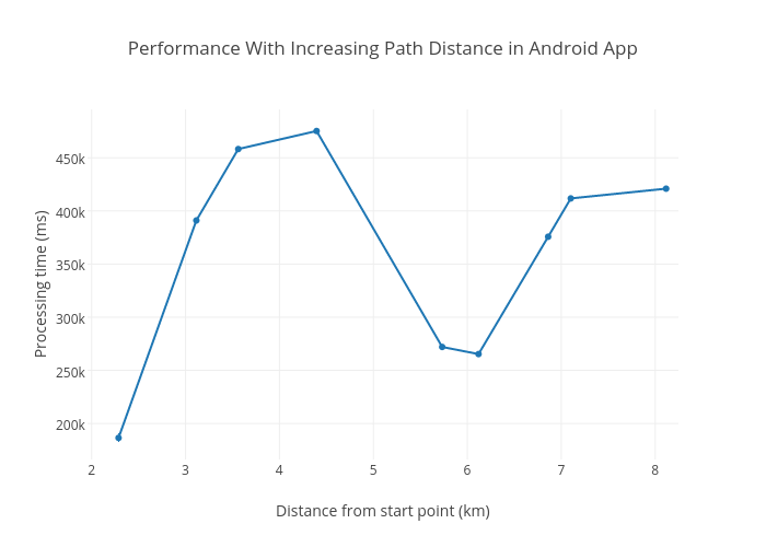
You are better off asking around which route to take than waiting 7 minutes for phone to calculate the best path. The performace was terrible, expecially in low end devices. I figured moving the path selection code to a Jersey web service running in a Digital Ocean VPS. My idea was to run the path centrally as the web service with the Android app acting only as a frontend. Sometimes all you need to do is throw a faster CPU and more RAM at your problem. The specifications for the VPS are:

OS: Ubuntu 14.04 x64

CPU: Intel(R) Xeon(R) CPU E5-2630L v2 @ 2.40GHz

Cores: 1

RAM: 512Mb

Porting the code was very easy. I was getting identical results from the path selection code running on the Android app and the web service, although much faster in the web service–twenty times faster actually.

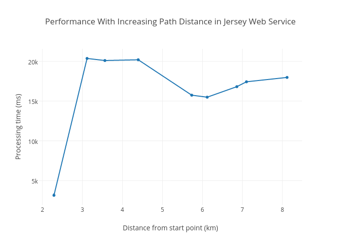
From both the Android and Jersey web service graphs, you can tell the algorithm scales really well with path complexity. Past some complexity, the processing time levels out. My focus shifted from scaling on path complexity to scalling to the number of concurrent requests the web service could handle mainly since we were no longer using a distributed processing model.

To test how the web service handled concurrent request, I used a tool called Siege. Here’s a sample siege sending 88 concurrent requests to the web service.

siege -b -r1 -c88 "http://api.ma3map.org/get/paths?from=-1.264945,36.721226&to=-1.281226,36.822575"

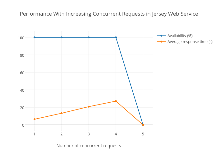
Up to 4 concurrent requests, the web service handles really well. However, you’ll notice that the response time rises at a rate of 7.5 seconds with every extra request. At 5 concurrent requests, the availability drops to 0. It would be really hard to make that work in production, especially due to the fact that requests in my use-case are expected to be in pulses (during rush hours). I had to either improve the algorithm in some way, I still don’t know how to, or adopt a different way of calculating the best path.

A colleague of mine introduced me to Neo4J around the same time I was grappling with the problem of scaling the Jersey Webserver. A graph database (such as Neo4J) would work! At the time, I didn’t know if it would have been faster but I was willing to try. I created a graph database with the stops as nodes and edges constructed between two nodes if these nodes share routes or are within a 2KM walking distance from each other. Path selection would involve simply querying the database for a path between the starting stop and the destination stop in the graph. It worked and it was fast, much faster than the web service. I installed the Neo4J database in the same VPS running the Jersey web service.

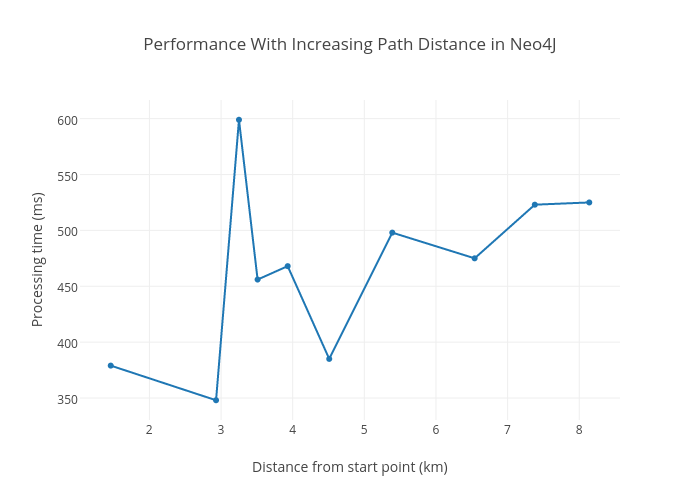
It scales well to path complexity, leveling out past some complexity. Did it however scale well to increasing concurrent requests? I performed the same siege test on the Neo4J database and the results were really impressive.

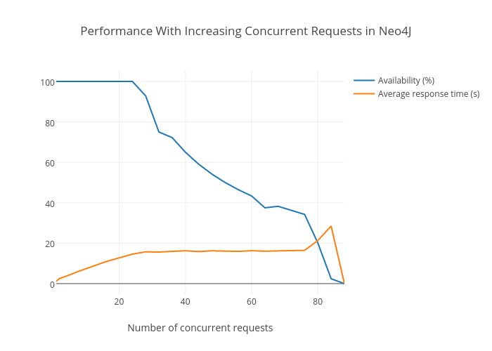
The graph maintained 100% availability up to 24 concurrent requests. It however did not dip to 0 at 25. The availability gradually decreased and finally zeroed out at 88 concurrent requests. What’s interesting here is that although the availability slowly decreased, the average response time for successfull requests leveled out at 16 seconds. This is awesome.

The graph database, however, still has some issues:

1. It’s not as accurate as the web service.
2. I am still unable to use a generated graph more than once. I have to regenerate the graph every time I bring up the API that wraps around it.

The next steps for me (after I solve these issues) will be to add more capabilities into the graph. Using metrics like traffic information to determine the best path is an example. The code is here. I wouldn’t mind more contributors!